3.0 Geometry Input
On the Geometry Input screen the user can define the room, fenestration and any object geometry and can access Advanced Options, the Material Database and Electric lighting input if desired, see the screenshot to the right. SPOT does not requires electric lighting input for daylighting analysis.
However, you will not be able to continue to the photosensor analysis portions of the program without electric lighting information. SPOT’s geometric modeling capabilities are somewhat limited to simpler spaces however new features allow for sloping of the ceiling, the addition of monitors, and the addition of any number of rotatable “block” objects that can be used to model a variety of daylighting, walls, and furniture elements. A Sketchup geometry import tool can be used behind the scenes and will be accessible in the interface soon.
The Spatial Characteristics section is used to define the general geometric dimensions and features of the space as well as the solar orientation and space height.
The Apertures and Objects section is used to define any fenestration in the model and blocks that can be used for any number of elements from overhangs, to cubicle walls, to exterior buildings, to core non-daylit spaces.
At any time while defining the model geometry, the Run Interactive View button can be used to display a quick interactive rendering of the current model in a viewing program called “rvu”. This is helpful to ensure the space has been modeled as intended. The image starts very crude and pixelated, but continually refines its resolution until a recognizable image is obtained, see rendering to the right. From this interactive viewer, any number of other Radiance views can be defined and implemented behind the scenes. A copy of the Radiance documentation for “rvu” is available here.
The Advanced Options button activates the Advanced Options screen which allows the user to change a number of the program calculation settings.
The Materials button opens the Material Database screen which allows the user to define a number of different material types for use in the SPOT model.
The Electric Lighting button opens the Electric Lighting input screen which allows the user to select luminaires from a database or import new luminaires and layout zones of electric lighting in the SPOT model.
The Back button will take you back to the Project Setup screen. If the project name and directory stay the same you can hit the Begin Project button and return right back to the Geometry screen and continue where you left off. This button can be useful to create a duplicated model. At any point after creating some geometry, the user can save the current project, and then return to the Project setup screen, change the project name, and create a duplicate model. This is useful when comparing the performance between several similar designs.
The Next button will take you to the Site and Schedule setup screen. If Electric Lighting calculations are desired, use the Electric Lighting button to access the Electric Lighting input screen.


3.1 Advanced Options
The Advanced Options button activates the Advanced Options screen, shown to the right, which allows the user to change a number of the program calculation settings. The program’s default values for each setting are listed and an input field allows the user to override each setting.
Calculations – These fields allow the user to override basic calculation settings.
Shading Devices – These fields allow the user to override the shading device settings.
Energy Model Schedule – This field allows users to pre-select a DOE-2 “include” file (*.inc) or Energy Plus 8760 text array to be exported in the analysis portion of the program. These files give an annual lighting power density (LPD) schedule(s) from results based on the SPOT schedule and photosensor control settings that can be used directly in DOE-2 or Energy Plus. Care should be taken to ensure the same weather files (TMY2 or EPW) files have been used and that the occupancy schedules and LPDs match between the energy simulation and the SPOT simulation.
Type 1 – Combines ON electric lighting zones and controlled electric lighting zones into two separate groups, resulting in two exportable include files.
Type 2 – Separates each electric lighting zone into its own exportable include file.
Type 3 – Combines all electric lighting zones into one schedule and one exportable include file.
Radiance Parameters – These fields allow the user to override the default Radiance parameters used for calculations and for renderings.
rvu Operation – Information on how to operate the rvu Radiance interactive viewer.
The Back button takes you back to the Geometry Input page.

3.1.1 Calculations
Months – This field allows the user to specify which months of the year to use for the design daylighting calculations. This field must include the solstices: December (12) for winter solstice and June (6) for the summer solstice and it must only contain months between December and June (ie. 12, 1, 2, 3, 4, 5, 6). If design results for a fall month are desired, choose the corresponding spring month. The months should be entered without quotes and separated by a comma.
Design Start Time – This field indicates the first time that will be calculated for each day selected.
The time must be an integer and input in 24 hour clock form. This start time is only used in the design
calculations, the annual calculations will be performed for hours between sunrise and sunset.

Design Stop Time – This field is the last time that will be calculated for each day selected. The time must be an integer and input in 24 hour clock form. This stop time is only used in the design calculations, the annual calculations will be performed for hours between sunrise and sunset.
Design Time Step – This field is the time step between calculation times for the design calculations only. The times calculated will always include noon, 12:00PM, and will vary off noon by this time step. The start and stop times will always be calculated.
Analysis Time Step – This field is the time step between calculation times for the analysis calculation matrix. The times calculated will always include noon, 12:00PM, and will vary off noon by this time step. The start and stop times are sunrise and sunset times for the analysis calculation matrix. Note that every time specified on the “Site and Usage Input” sheet are still calculated for the annual simulations, interpolated as necessary from the analysis calculation matrix.
Create Renderings – This field requires either Yes (Y) or No (N) and tells SPOT whether or not to perform renderings of the space. If this option is selected the renderings will begin simulating upon getting to the Photosensor Generator page and they will be viewable while on the Calculating page. The rendering can be viewed on the Calculating page even if not selected to pre-calculate on the Advanced Options page however the user will have to wait at that time for the renderings to finish.
Field Point Spacing – This field allows the user to specify the spacing distance to use for the calculation grids. If left empty, the program will auto-size the calculation grid to fit the defined geometry width and length. Typically auto-sizing will result in a grid with between 10 and 15 rows and columns. WARNING – A small grid size for a large space will result in a large calculation grid and long calculation times. See the Photosensor Generator section for grid size limitations.
Field Wall Spacing – This field defines the offset the calculation grid will have from the walls of the space. The default offset is 2 feet or 0.5 meters.
Equinox 9am and 3pm? – This field forces SPOT to calculate the Equinox at 9am and 3pm times, regardless of the other time step, start and stop time settings. These times are commonly needed for LEED and other daylight metrics.
3.1.2 Shading Devices
The fields in the Window Type Definition area define the parameters that will be used for the various windows in your SPOT project. The input fields are shown to the right and discussed below.
Window Type # – This pulldown menu selects the current window type # (1-10). SPOT allows you to define the following information for up to 10 different types of windows. This is useful when there are multiple types of windows and/or skylights on your project with different base parameters. All the types will default to the same default, so if no additional types (beyond 1) are defined, SPOT will use this type for all windows. If more than 1 type is defined differently then the defaults, you will have the option to assign a window type to each window defined in your model in the Apertures and Objects input section.
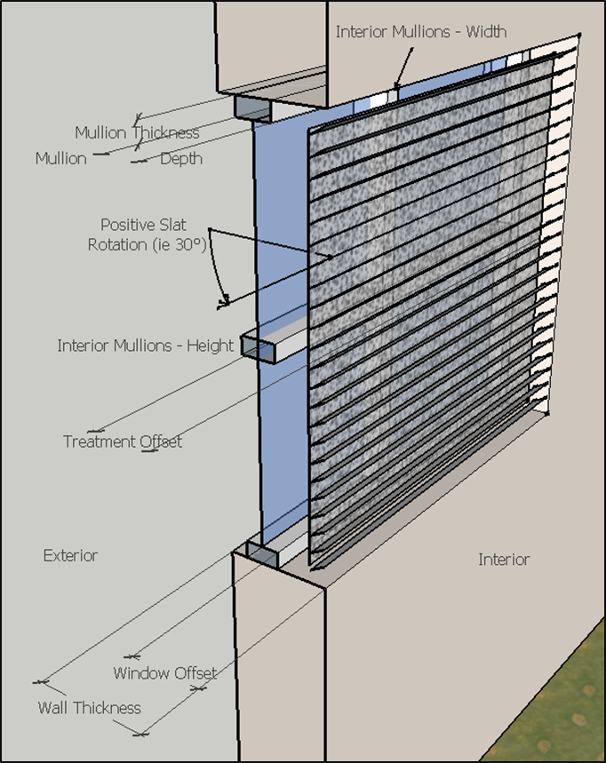
Blind Slat Rotation – This field sets the rotation angle of any blinds used in this window type. Open slats, perpendicular to your window, would have a 0° rotation and a positive number rotates the inside slat edge down.
Blind Slat Width – This field sets the width, and spacing, of any blinds used in this window type. Typically, blinds are between 1 and 2” wide, but a larger 9” or 12” louver can also be defined.
Mullion Thickness – This defines the thickness of the window frame in this window type. This is the distance that the actual glass will be offset from the window opening in the wall.
Mullion Depth – This defines the depth of the window frame in this window type. Many typical store front systems will be 4.5” – 6” but they can vary, particularly with larger curtain wall systems. Caution, if this is defined deeper than the window thickness or offset enough, it will stick out of the edge of the wall.
Interior Mullions – Width – This defines the number of interior mullions across the width of the window. A value of 0 would have no intermediate mullions, a value of 1 would model one vertical mullion, centered along the width of the window, and so on.
Interior Mullions – Height – This defines the number of interior mullions across the height of the window. A value of 0 would have no intermediate mullions, a value of 1 would model one horizontal mullion, centered along the height of the window, and so on.
Window Mounting Location – This defines where the glass is mounted relative to the window frame. Three mounting options are available: ‘i’ for interior mounting, ‘c’ for a centered mounting, and ‘e’ for an exterior mounting. Interior will place the glass flush with the interior edge of the window frame. Center will center the glass in the window frame. Exterior will place the glass flush with the exterior edge of the window frame.
Window Offset – This defines the distance between the pane of glass and the interior wall surface.
The window frame will be moved and placed accordingly. This must be less than the wall thickness.
Window Treatment Offset – This defines the distance between the glass and any interior or exterior
shading devices. For blinds, it defines the plane that contains the exterior edge of the blinds.
A positive values defines interior treatment, while a negative value can define an exterior blind or shade.
Selecting the Check Mark button displays the illustration to the right that diagrams what each window and shading parameter controls.
The Miscellaneous Simulation Settings area defines the manual control setting for all window types and the energy modeling schedule type.
Manual Shade Control Delay – This defines how many hours past a window glare incident in which a user would reopen manual shades or blinds. 4 hours might be the most typical occupant. 3 hours represents a fairly aware occupant. A more active occupant might readjust blinds after 2 hours. Even the most conscious occupant, rarely readjusts blinds every hour.
Manual Shade Glare Trigger – This defines the exitance threshold of a window before it represents a potential source of glare. An exitance of 500fc gives a reasonable approximation.
Energy Model Schedule Type – This defines the method to use when writing out Lighting Power Density modifier schedules for either DOE-2 or EnergyPlus.

3.1.3 Radiance Parameters
The user can use the Quality, Detail and Variability settings to control all the Radiance parameters or change each parameter individually. For most cases, the default settings of (M)edium M M, will give results accurate to +/-20% and is good for initial evaluation of a space. However, for accurate reports and design comparisons, a Variability setting of (H)igh is recommended and required for valid reports. The renderings with these settings might still be a bit splotchy but will give a sense of the daylight distribution. Setting Quality and Variability to H will result in better renderings and more accuracy overall at the cost of increased time. A Detail setting of M is usually sufficient for most spaces. However, if there is a lot of detail due to many smaller windows or many small or skinny block objects, then Detail should be set to H for better accuracy and renderings. Use caution whenever changing Radiance parameters, they can greatly influence the simulations time and accuracy.
Note, any time BSDF files are used and represent a significant source of light into the space, higher Radiance ambient parameters are typically required to maintain accuracy: particularly the ambient division (-ad) parameter should be set rather high at 4096 or 8192. The program will detect when these are used and automatically set -ad to 4096.
Copied from the Radiance manual for rpict, below are descripitions of the various Radiance parameters:
-dj frac Set the direct jittering to frac. A value of zero samples each source at specific sample points (see the −ds option below), giving a smoother but somewhat less accurate rendering. A positive value causes rays to be distributed over each source sample according to its size, resulting in more accurate penumbras. This option should never be greater than 1, and may even cause problems (such as speckle) when the value is smaller. A warning about aiming failure will issued if frac is too large.
-ds frac Set the direct sampling ratio to frac. A light source will be subdivided until the width of each sample area divided by the distance to the illuminated point is below this ratio. This assures accuracy in regions close to large area sources at a slight computational expense. A value of zero turns source subdivision off, sending at most one shadow ray to each light source.
-dt frac Set the direct threshold to frac. Shadow testing will stop when the potential contribution of at least the next and at most all remaining light sources is less than this fraction of the accumulated value. (See the −dc option below.) The remaining light source contributions are approximated statistically. A value of zero means that all light sources will be tested for shadow.
−dc frac Set the direct certainty to frac. A value of one guarantees that the absolute accuracy of the direct calculation will be equal to or better than that given in the −dt specification. A value of zero only insures that all shadow lines resulting in a contrast change greater than the −dt specification will be calculated.
-dr N Set the number of relays for secondary sources to N. A value of 0 means that secondary sources will be ignored. A value of 1 means that sources will be made into first generation secondary sources; a value of 2 means that first generation secondary sources will also be made into second generation secondary sources, and so on.
-dp D Set the secondary source presampling density to D. This is the number of samples per steradian that will be used to determine ahead of time whether or not it is worth following shadow rays through all the reflections and/or transmissions associated with a secondary source path. A value of 0 means that the full secondary source path will always be tested for shadows if it is tested at all.
-ss samp Set the specular sampling to samp. For values less than 1, this is the degree to which the highlights are sampled for rough specular materials. A value greater than one causes multiple ray samples to be sent to reduce noise at a commmesurate cost. A value of zero means that no jittering will take place, and all reflections will appear sharp even when they should be diffuse.
-st frac Set the specular sampling threshold to frac. This is the minimum fraction of reflection or transmission, under which no specular sampling is performed. A value of zero means that highlights will always be sampled by tracing reflected or transmitted rays. A value of one means that specular sampling is never used. Highlights from light sources will always be correct, but reflections from other surfaces will be approximated using an ambient value. A sampling threshold between zero and one offers a compromise between image accuracy and rendering time.
-av red grn blu Set the ambient value to a radiance of red grn blu . This is the final value used in place of an indirect light calculation. If the number of ambient bounces is one or greater and the ambient value weight is non-zero (see -aw and -ab below), this value may be modified by the computed indirect values to improve overall accuracy.
-aw N Set the relative weight of the ambient value given with the -av option to N. As new indirect irradiances are computed, they will modify the default ambient value in a moving average, with the specified weight assigned to the initial value given on the command and all other weights set to 1. If a value of 0 is given with this option, then the initial ambient value is never modified. This is the safest value for scenes with large differences in indirect contributions, such as when both indoor and outdoor (daylight) areas are visible.
-ab N Set the number of ambient bounces to N. This is the maximum number of diffuse bounces computed by the indirect calculation. A value of zero implies no indirect calculation.
-ar res Set the ambient resolution to res. This number will determine the maximum density of ambient values used in interpolation. Error will start to increase on surfaces spaced closer than the scene size divided by the ambient resolution. The maximum ambient value density is the scene size times the ambient accuracy (see the −aa option below) divided by the ambient resolution. The scene size can be determined using getinfo(1) with the −d option on the input octree.
-aa acc Set the ambient accuracy to acc. This value will approximately equal the error from indirect illuminance interpolation. A value of zero implies no interpolation.
-ad N Set the number of ambient divisions to N. The error in the Monte Carlo calculation of indirect illuminance will be inversely proportional to the square root of this number. A value of zero implies no indirect calculation.
-as N Set the number of ambient super-samples to N. Super-samples are applied only to the ambient divisions which show a significant change.
3.1.4 rvu Operation
The following are the rvu instructions from the Radiance manual. The rvu program used in SPOT has been compiled on Windows by NREL. It has one bug in the saving of images or view files. When using the pull-down menus, the image save and view file save functions cannot correctly read spaces in either the file name or in the target directory. To get around this you can manually type in the commands in the command window. Some common helpful tasks are:
Save current view – type “view views/[viewfilename]” to save a current view into the views directory. These typically have a *.vf (view file) or a *.vp (view point) file extension.
Save current image – type “write images/[imagefilename]” to save the current image into the projects images directory. These should have a *.hdr (high dynamic range) file extension.
Load saved view – type “last views/[viewfilename]” to load a saved view. SPOT automatically generates 8 views for every model: four perspective views at each corner (sw.vf, se.vf, nw.vf, and ne.vf) and four section views on each side (Wsect.vf, Ssect.vf, Esect.vf, Nsect.vf). The southwest perspective view is automatically loaded, but other views can easily be loaded by typing “last views/Wsect.vf” for example.
Change aim of current view – type “aim” and then click on the image where you want the new center of view.
Move view location – press the X,Y,Z arrow buttons to move the view location.
NAME
rvu – generate RADIANCE images interactively
SYNOPSIS
rvu [ rpict options ][ −n nproc ][ −o dev ][ −b ][ −pe exposure ][$EVAR ][@file ] octree
rvu[options ] −defaults
rvu−devices
DESCRIPTION
Rvu generates RADIANCE images using octree. (The octree may be given as the output of a command enclosed in quotes and preceded by a ‘!’.) Options specify the viewing parameters as well as giving some control over the calculation. Options may be given on the command line and/or read from the environment and/or read from a file. A command argument beginning with a dollar sign (’$’) is immediately replaced by the contents of the given environment variable. A command argument beginning with an at sign (’@’) is immediately replaced by the contents of the givenfile. The options are the same as for rpict(1), with a few notable exceptions. The −pd, −r,−z, −S, −P,−PP and −t options are not supported, and −o specifies which output device is being used instead of the output file. The −x, −y and −pa options are unnecessary, since rvu scales the display image to the specified output device. Additionally, the −b option improves the display on greyscale monitors, and −pe may be used to set an initial exposure value.
The −n option may be used to specify multiple processes, to accelerate rendering.
In the second form, the default values for the options are printed with a brief explanation. In the third form, the list of supported output devices is displayed.
rvu starts rendering the image from the selected viewpoint and gradually improvesthe resolution of the display until interrupted by keyboard input. rvu then issues a prompt (usually ’:’) and accepts a command line from the user. rvu may also stop its calculation and wait for command input if the resolution of the display has reached the resolution of the graphics device. At this point, it will give the ’done:’ prompt and await further instructions. If rvu runs out of memory due to lack of resources to store its computed image, it will give the ’out of memory:’ prompt. At this prompt, the user can save the image, quit, or evenrestart a new image, although this is not generally recommended on virtual memory machines for efficiencyreasons.
rvu is not meant to be a rendering program, and we strongly recommend that rpict(1) be used instead for that purpose. Since rpict(1) does not store its image in memory or update anydisplay of its output, it is much faster and less wasteful of its resources than rvu. rvu is intended as a quick interactive program for deciding viewpoints and debugging scene descriptions and is not suited for producing polished images.
COMMANDS
Once the program starts, a number of commands can be used to control it. A command is given by its name, which can be abbreviated, followed by its arguments.
aim [mag [ x y z ] ]
Zoom in by mag on point xyz. The view point is held constant; only the view direction and size are changed. If xyz is missing, the cursor is used to select the view center. A negative magnification factor means zoom out. The default factor is one.
ˆC Interrupt. Go to the command line.
exposure [spec ]
Adjust exposure. The number spec is a multiplier used to compensate the average exposure. A value of 1 renormalizes the image to the computed average, which is usually done immediately
after startup. If spec begins with a ’+’ or ’-’, the compensation is interpreted in f-stops (ie. the power of two). If spec begins with an ’=’, an absolute setting is performed. An ’=’ by itself permits interactive display and setting of the exposure. If spec begins with an ’@’, the exposure is adjusted to present similar visibility to what would be experienced in the real environment. If spec is absent, or an ’@’ is followed by nothing, then the cursor is used to pick a specific image location for normalization.
focus [distance]
Set focus distance for depth-of-field sampling. If a distance in world coordinates is absent, then the cursor is used to choose a point in the scene on which to focus. (The focus distance setting does not affect rendering in rvu, butcan be used in rpict with the −pd option to simulate depth-of-field on views savedfrom rvu.)
frame [xmin ymin xmax ymax ]
Set frame for refinement. If coordinates are absent, the cursor is used to pick frame boundaries. If ‘‘all’’ is specified, the frame is reset to the entire image.
free Free cached object structures and associated data. This command may be useful when memory is lowand a completely different viewisbeing generated from the one previous.
last [file ] Restore the previous view. Ifavieworpicture file is specified, the parameters are taken from the last view entry in the file.
L [vw[rfile ] ]
Load parameters for view vw from the rad(1) input file, rfile. Both vw and rfile must be given the first call, but subsequent calls will use the last rfile as a default, and “1” as the default view (ie. the first viewappearing in rfile). If rvu wasstarted by rad, then the rfile parameter will initially default to the rad input file used.
move [mag [ x y z ] ]
Move camera mag times closer to point xyz. Foraperspective projection (or fisheye view), only the viewpoint is changed; the viewdirection and size remain constant. The viewsize must be modified in a parallel projection since it determines magnification. If xyzis missing, the cursor is used to select the viewcenter.Anegative magnification factor decreases the object size. The default factor is one. Care must be taken to avoid moving behind or inside other objects.
new [nproc ]
Restart the image, using the specified number of rendering processes. Usually used after the “set” command.
origin ]
Change vieworigin to the indicated world position xo yo zo looking in the direction xd yd zd. If the direction is missing, the current viewdirection is used. If the origin is missing, the cursor is used to select the vieworigin, and the direction will be determined by the (reoriented) surface normal. The viewtype and size will not be altered, but the up vector may be changed if the newdirection coincides.
pivot angle [ elev[mag [ x y z ] ] ]
Similar to the “move“command, but pivots the viewabout a selected point. The angle is measured in degrees around the viewupvector using the right hand rule, so a positive value pivots the viewer to the right of the selected point. The optional elev is the elevation in degrees from the pivotpoint; positive raises the viewpoint to look downward and negative lowers the view point to look upward.
quit Quit the program.
ˆR Redraw the image. Use when the display gets corrupted. On some displays, occassionally forcing a redrawcan improve appearance, as more color information is available and the driver can makeabetter color table selection.
rotate angle [ elev[mag ] ]
Rotate the camera horizontally by angle degrees using the right-hand rule. A positive value rotates the viewtow ards the left, and a negative value looks to the right. If an elevation is specified, the camera looks upward elev degrees. (Negative means look downward.)
set [var [ val ] ]
Check/change program variable. If var is absent, the list of available variables is displayed. If val is absent, the current value of the variable is displayed and changed interactively. Otherwise, the variable var assumes the value val. Variables include: ambient value (av), ambient value weight (aw), ambient bounces (ab), ambient accuracy(aa), ambient divisions (ad), ambient radius (ar), ambient samples (as), black&white (b), back face visibility (bv), direct jitter (dj), direct sampling (ds), direct threshold (dt), direct visibility (dv), irradiance (i), limit weight (lw), limit recursion (lr), medium extinction (me), medium albedo (ma), medium eccentricity (mg), medium sampling (ms), pixel sample (ps), pixel threshold (pt), specular jitter (sj), specular threshold (st), and uncorrelated sampling (u). Once a variable has been changed, the “new” command can be used to recompute the image with the newparameters. If a program variable is not available here, it may showupunder some other command or it may be impossible to change once the program is running.
trace [xbegybegzbegxdir ydir zdir ]
Trace a ray. If the ray origin and direction are absent, the cursor is used to pick a location in the image to trace. The object intersected and its material, location and value are displayed.
view [file [ comments ] ]
Check/change view parameters. If file is present, the view parameters are appended to a file, followed by comments if any. Alternatively, viewoptions may be given directly on the command line instead of an output viewfile. Otherwise, viewparameters are displayed and changed interactively.
V [vw[rfile ] ]
Append the current viewasview vw in the rad file rfile. Compliment to L command. Note that the viewissimply appended to the file, and previous views with the same name should be removedbefore using the file with rad.
write [file ]
Write picture to file. If argument is missing, the current file name is used.
ˆZ Stop the program. The screen will be redrawn when the program resumes.
ENVIRONMENT
RAYPATH the directories to check for auxiliary files.
DISPLAY_GAMMA the value to use for monitor gamma correction.
AUTHOR
GregWard
SEE ALSO
getinfo(1), lookamb(1), oconv(1), pfilt(1), rad(1), rpict(1), rtrace(1)
3.2 Material Database
The Materials button will take you to the Material Database screen, shown to the right. This screen allows the user to define a number of different material types for use in your SPOT model.
In the Material Library Editor section, there are existing libraries of materials to choose from with the ability to add new libraries and new materials. You can also render the material to see how it may appear in the final SPOT model.
In the Project Materials and Surface Assignment section, the user adds materials to the current project from these libraries and can then assign them to the various elements of the SPOT model.

3.2.1 Material Library Editor
This section is where you can choose materials from the libraries, modify them as necessary, create new libaries and materials, and render them to see how they may appear in a Radiance model.
Libraries
The scroll window displays all the current libraries available to choose materials from. Select a libary and it’s material contents will be displayed in the Materials window to the right. The New Library button will bring up a window to enter the New Library Name. This will create an empty library with the given name. The Import Library button will bring up an import window asking for the name of a Radiance library to import. This can be any text file that has valid (and SPOT supported) Radiance material definitions. See below for the types of materials SPOT currently supports. The Delete Library button will delete the currently selected Library.
Materials
The scroll window displays all the available materials in the currently selected library. Select a material and the material details will show up in the Material Editor section below. The New Material button clears the Material Editor fields so the user can input custom material information and save into a library. The Save Material button will then save a new, or modified, material definition with the current material name (note that no spaces can exist in the name) back to the current library. This can be used for new materials or for modifying, or ‘cloning’, existing materials. For this, just pull up an existing material, modify as necessary and either hit save with the same name to Modify the material or change the name and save to create a clone of the material. The Delete Material button will delete the currently selected material.

Material Editor
These fields allow you to access the details of any material or pattern. The Render button will run a quick Radiance simulation and display an image of the currently selected material on a sphere. This best shows what the material may look like in a Radiance model under the variable lighting and shadow that will exist. The Import to Project button will import the currently selected material to the project list. Only materials that have been imported to the project can then be applied to a surface in your SPOT model. The different material and pattern types are available and their control parameters are discussed below:
Plastic – This material type is most common and can model most opaque surfaces that do not have unique specularity characteristics like those of metals or assymetric surfaces. It is a material with uncolored highlights. The following 5 parameters control the appearance:
Red refl, Green refl, Blue refl – These fields set the RGB reflectance of the material.
Specularity – This field sets the fraction of the reflectance that is specular in nature. Most materials have a specularity fraction less than 0.1.
Roughness – This field sets the roughness value of the surface. A value of 0 is a perfectly smooth surface. A value of 0.2 is a fairly rough surface and roughness values greater than 0.2 are uncommon.
Metal – This material type is similar to plastic except the specular highlights are modified by the material color. The following 5 parameters control the appearance:
Red refl, Green refl, Blue refl – These fields set the RGB reflectance of the metal. These will affect both the diffuse and specular reflectance.
Specularity – This field sets the fraction of the reflectance that is specular in nature. Most metals have a specularity fraction greater than 0.9.
Roughness – This field sets the roughness value of the surface. Values greater than 0.2 are uncommon.
Glass – This material type as the name suggests is for modeling thin glass surfaces with an index of refraction of 1.52 (n = 1.52). The following 3 parameters control the appearance.
Red trans, Green trans, Blue trans – These fields set the RGB transmissivity of the glass. Transmissivity is the amount of light not absorbed in one traversal of the material. Transmittance, the value usually measured, is the total light transmitted through a pane including reflections.
To compute transmissivity (tn) from transmittance (Tn) use: tn=(sqrt(0.8402528435+.0072522239xTnxTn)-.9166530661/.0036261119/Tn
Trans – This material type is for modeling translucent (diffusing) transmissive materials. These materials can have a reflective and absorbtive component as well. The total Transmittance (specular and diffuse), Reflectance (specular and diffuse) and Absorbtance must be equal to 1 to ensure conservation of energy. The following 9 parameters control the appearance:
Diffuse Refl – This field defines the diffuse reflectance of the material.
Specular Refl – This field defines the specular reflectance of the material.
Absorbtance – This field defines the absorbtance of the material.
Diffuse Trans – This field defines the diffuse transmittance of the material.
Specular Trans – This field defines the specular transmittance of the material.
Roughness – This field defines the surface roughness. A value of 0 is a smooth surface and is necessary if a specular transmittance (view) component is desired such as the case with bug screens or fabric meshes. A value of 0.2 represents a fairly rough surface.
Red Ratio, Green Ratio, Blue Ratio – These fields define the relative color of the material. These can be entered as any value – the relative relationship is what matters.
Mirror – This material type is for modeling perfectly specular mirrors that will be considered in the direct calculation in Radiance as virtual secondary sources. The following 3 parameters control the appearance:
Red refl, Green refl, Blue refl – These fields set the RGB 100% specular reflectance of the material.
BSDF – This material type is for modeling surfaces that scatter the transmitted and/or reflected light and can be described with a Bi-Directional Scatter Distribution Function (BSDF) file. SPOT Pro uses the standard .xml format defined by Lawrence Berkley National Labs and used in the Windows 7.0 and Radiance software. The following 5 parameters control the appearance:
Thickness – This field defines the overall thickness of the geometry being represented by the BSDF file. If the BSDF file represents a planar system this should be left at 0 which means the BSDF file will be applied to a plane and will will interact with both the direct and ambient calculations in Radiance. If it is a “System BSDF” file and represents a larger optical system than the thickness should represent the distance between an output plane (where daylight enters the space) and an input plane (where daylight is collected) of the system. The system will be modeled with the given depth in Radiance. Care should be taken to ensure the roof depth is as desired, so that the system is not modeled recessed into the roof or ceiling.
XML File – This field defines the name of the XML file to use. The file will need to be provided separately (SPOT does not generate an XML file currently) and will need to be manually copied to the XML directory located at C:\SPOT\materials\xml for the material to work correctly.
Orientation X, Orientation Y, Orientation Z – These fields define the orientation of the XML file. This is the orientation of the +Y vector when using genBSDF to create the BSDF file. The orientation vector is typically up (0,0,1) for side daylighting products and usually north (0,1,0) for top daylighting products.
Sys.Trans – This field is only used if the BSDF file has a thickness. In this case, the BSDF file does not directly affect the direct calculations and so a proxy geometry is created in between the systems’ input and output planes that will have this approximate effective transmittance when dealing with the direct calculation. This should be approximately the systems hemispherical transmittance.
Corrugate – This is a pattern type for modeling an undulating surface like a corrugated metal deck. The following parameters control the appearance:
Direction [X, Y, Z] – This sets the direction of the corrugation. A setting of X will make all the ridges run perpendicular to the X axis and so forth.
Magnitude [0 – 1] – This sets the magnitude of the corrugation. A value of 0 would be a perfectly smooth surface and a value of 1 would make the height of the corrugations match the spacing of the corrugations.
Frequency [>0] – This sets the frequency of the corrugation. The value sets the number of times the material oscillates in 1 meter.
Perforate – This is a pattern type for modeling perforated surfaces like punched metals or glass pv products. The following 6 parameters control the appearance:
Openness [0-1] – This sets the openness (or coverage in the case of an opaque hole material) of the overall perforation pattern. A value of 0 will make no holes/dots, (would be all base material, and a value of 1 would be all hole/dot material.
Scale [>0] – This sets the overall scale of the perforation relative to 1 meter square. For example, a value of 0.1 would make a pattern of 10 perforated holes/dots per 1 meter of material.
Shape [Round,Square] – This sets the shape of the perforated holes/dots to be either circular or square. The perforation pattern is not offset from row to row or column to column and so makes a uniform pattern of the holes/dots.
Base Material – This sets the base material to use. This is the material that will used when the perforation pattern is not making holes or dots This material can be void or a glass if the perforation is a pattern of dots or an opaque material such as a frit.
Hole/Dot Material – This sets the hole/dot material to use. This material will be used when the perforation pattern is indicating a hole or dot.
Surface [X, Y, Z] – This sets the orientation of the holes. Choose X if you want the holes/dots to be punched in the X direction and so forth.
Brick – This is a pattern type for modeling brick or tile patterns. The following 8 parameters control the appearance:
Grout Width [>0] – This defines the width of grout between each brick in meters. A value of 0.01 gives a 1cm grout.
Brick Height [>0] – This defines the height of each brick in meters.
Brick Width [>0] – This defines the width of each brick in meters.
Offset [>0] – This defines the offset between two adjacent rows of bricks. A value of 0 would align the bricks creating a uniform grid or tile pattern. A value equal to 1/2 of the brick width would offset each row of bricks by 1/2 of the brick width creating a typical brick pattern.
Brick bright [1 +/-] – This defines the relative brightness of the bright pattern. As this pattern is applied to a surface that will also have a material applied to it, this will adjust that materials reflectance up or down by this multplier to create the brick pattern.
Grout bright [1 +/-] – This defines the relative brightness of the grout. As this pattern is applied to a surface that will also have a material applied to it, this will adjust that materials reflectance up or down by this multplier to create the grout lines.
Surface [Vert, Horiz] – This defines whether the brick pattern will be on a horizontal surface or a vertical surface. Tile floor patterns would typically be applied to a horizontal surface where as brick patterns may typically be applied to a vertical surface.
Scale [>0] – This defines the overall scale of the brick pattern. A value of 1 means the base unit is 1 meter and the width and height inputs above are in units of a meter. Any other value adjusts these other parameters relatively and can be used to create larger or smaller patterns without adjust each individual parameter.
3.2.2 Project Materials and Surface Assignment
The left side of the Materials screen lists the current project materials and the surface material assignments.
Project Materials – This window lists the current materials that have been imported into the project and are available to be applied to a surface. Select a material by right-clicking it in the list. The Delete button will delete the currently selected material from the project list only, not the library it may have come from.
The Assign Material to Object button will assign the currently selected material in the project list to the currently selected row in the Surface Material Assignment section.
Surface Material Assignment – This window lists the current elements in the project (Object column), the associated materials (Material column) and any associated patterns or textures (Patterns/Textures column). The default materials are grey-scale with the visible reflectance specified in the Material input field. Anytime a 0-100 number is specified in the Material column, SPOT will assume this to be a grey surface with the given percentage transmittance. (ie. 35 will give a gray surfaced with a 35% reflectance). Otherwise, the Material input should contain the name of a valid material that has been added to your project. The Patterns/Textures column should either be blank or contain the name of a valid pattern or texture material that has been added to the project. When a project geometry is imported, any number of project elements may exist in the Object column. Geometry created within SPOT will always contain the following elements:
Interior Walls – Interior surface of all walls
Exterior Walls – Exterior surface of all walls
Floor – The floor of the space.
Ceiling – Both regular and monitor ceiling
Roof – Typically not seen but can influence light entering clerestory windows
Mullions – Frame material of all windows
Ground – Exterior ground surface
Shades – Fabric shades
Blinds – Reflectance of slats, other parameters defined on Advanced Options.

3.3 Spatial Characteristics
This section defines the general geometric dimensions and features of the space as well as the solar orientation and space height. The figure to the right shows a screen shot of Spatial Characteristics input. The Compass window and the Isometric window are updated in real-time to give the user visual feedback of the geometry they are defining.
General Dimensions
Width – This field sets the overall width, or North-South dimension, of the space. The dimension measures from interior wall to interior wall.

Length – This field sets the overall length, or East-West dimension, of the space. The dimension measures from interior wall to interior wall.
Height – This field sets the overall height of the space from finished floor to finished ceiling. If a sloped roof is selected, this field will be ignored in lieu of the height defined for each corner.
Workplane Height – This field sets the location of the illuminance calculation grid above the finished floor. This can be any height within the limits of the space, but is typically used to represent a workplane, 30 – 36” above the finished floor.
Wall Thickness – This field sets the thickness of the exterior walls, and essentially defines the thickness of any window sills in the model. The window and window mullion (frame), as defined in the Shading Devices section of Advanced Options, will still exist inside of this window opening.
Roof Thickness – This field sets the depth of any skylight openings placed in the model, essentially the distance between the finished ceiling and the skylight opening to the sky. The shafts are assumed to be orthogonal. Splayed skylight shafts are not currently supported with the SPOT geometry modeler.
Sloped Ceiling? – This field determines whether the ceiling will be sloped or not. If (Y)es, the additional fields below will be visible and used to determine the ceiling height in the space in lieu of the height input above.
NW Height, NE Height, SE Height, SW Height – This field sets the height of the northwest, northeast, southeast, and southwest (respectively) corner of the space.
Splice Direction – If the 4 heights listed above are not co-planar, the the ceiling will be created with two triangles. This defines whether the splice between those two triangles takes the high path, or the low path.
Monitor Dimensions
Monitor? – This field determine whether a monitor, or raised roof section, exists in the model.
Currently, only one monitor can be used in a given model. If (Y)es, the additional fields below
will be visible and used to determine the monitor dimensions and ceiling height within the monitor.
Width – This field sets the overall width, or North-South dimension, of the monitor. The dimension measures from the interior of the monitor walls.
Length – This field sets the overall length, or East-West dimension, of the monitor. The dimension measures from the interior of the monitor walls.
Height – This field sets the overall height of the monitor from finished floor to finished ceiling. If a sloped monitor roof is selected, this field will be ignored in lieu of the height defined for each corner of the monitor.
Site and View
View Height – This field sets the camera angle for the isometric diagram. It is limited in range from 0° to 45°. Adjusting this angle can be helpful in viewing certain objects in your model that perhaps overlap at the given angle.
Orientation – This field sets the space’s orientation relative to true south. This input must be between –45° and 45°, since any rotation greater than 45° simply changes which façade is referred to as “South”. The compass window shows the user the orientation of the footprint of the space relative to the true cardinal directions. Throughout the program, the south façade is denoted as the orange façade, while all other facades are shown as blue.
Bldg Height – This field sets the space’s height relative to the ground plane outside.
0’ represents a bottom floor, where 15’ might represent a 2nd floor and 100’+ can be
used to represent a sky scraper space. A solid wall will be modeled below the space
model down to the ground plane to create the necessary shadows.
Wall to west? – This field defines exterior walls to the west of the building model. Two walls are placed in the same plane as the north and south walls of the model, with the same wall thickness and at the given distance to the west of the west wall. The walls will extend down to the ground plane that’s distance is defined by the Building Height value.
Wall to east? – This field defines exterior walls to the east of the building model. Two walls are placed in the same plane as the north and south walls of the model, with the same wall thickness and at the given distance to the east of the east wall. The walls will extend down to the ground plane that’s distance is defined by the Building Height value.

Dist from South – This fields sets the distance between the south wall and the south monitor wall, measured from the interior of both walls. The field must be greater than 0 and less than the space width minus the monitor width.
Dist from West – This fields sets the distance between the west wall and the west monitor wall, measured from the interior of both walls. The field must be greater than 0 and less than the space length minus the monitor length.
Wall Thickness – This field sets the thickness of the monitor walls, and essentially defines the thickness of the window sills. The window and window mullion (frame), as defined in the Shading Devices section of Advanced Options, will still exist inside of this window opening.
Monitor Sloped? – This field determines whether the monitor ceiling will be sloped or not. If (Y)es, the additional fields below will be visible and used to determine the ceiling height in the space in lieu of the height input above. This option can be used to create sawtooth monitor forms.
NW Height, NE Height, SE Height, SW Height – This field sets the height of the northwest, northeast, southeast, and southwest (respectively) corner of the monitor.
Splice Direction – If the 4 heights listed above are not co-planar, the ceiling will be created with two triangles. This defines whether the splice between those two triangles takes the high path, or the low path.

3.4 Apertures and Objects
The wall and aperture inputs, shown to the right, allow the user to define a number of architectural features for each façade of the space. The user selects which Surface to add architectural features to using the Surface pull-down menu. This menu contains an option for each of the four walls (east, south, west, and north), the roof, and one for each monitor wall if a monitor exists. Once a façade is selected, the user can define any number of windows or blocks on that facade. When the roof is selected, a reflected ceiling plan will be shown in the display window, as seen to the right, otherwise an interior elevation of the selected surface is shown.
Windows
The window inputs allow the user to define any number of window or skylights, as long as they fit, onto any surface of the model.
Window # – This pull-down menu indicates which window is currently being viewed. Each window defined is numbered starting with 1 and then 2, and so on. Up to 36 windows can be defined for each façade. Beyond this, it is possible to define more but the isometric and elevations will not display them due to limitations in excel.
Copy… – This pull-down menu allows the user to copy a window definition from a previously defined window. The copied window will appear directly on top of the original and will need to be moved to an available (non-overlapping) position.
Distance from Left Wall (Distance from West Wall) – This field sets the window’s distance from the left wall when viewed as an interior elevation or as a reflected ceiling plan. The scale on the interior elevation plot illustrates this dimension. When the roof surface is selected the value becomes the distance from west wall or the X distance, as seen in the Figure below.
X Location – This field defines the X location of the base corner of the current block.
Y Location – This field defines the Y location of the base corner of the current block.
Z Location – This field defines the Z location of the base corner of the current block.
The X, Y, and Z size inputs define the size of the block from the base corner defined above. Typically, these will be positive values, but negative values can be used and are sometimes more convenient.
X Size – This field defines the X size of the current block.
Y Size – This field defines the Y size of the current block.
Z Size – This field defines the Z size of the current block.
Reflectance – This field defines the reflectance of the current block. Alternatively, the name of a valid material that has been imported into the project on the Materials page can be input and will be used for the block.
Fixed to Surface – This field allows you to fix the defined block to the current surface it is being placed on. This is useful for objects that are often located relative to a surface and should move with that surface. For example, a lightshelf could be fixed to the Interior of an east surface and will move with that surface if the space length changes. A block can be fixed to the Exterior or Interior or a surface or set as Free (or left blank) to not move with a surface at all.
Rotation – This field defines the rotation of the current block in degrees around the blocks insertion point. The rotation is around the Z-axis of the model using the right-hand rule (counter-clockwise from above) for positive angles. This field can be left blank for no rotation.
At any time, you can use the Delete button to remove the selected block. All the blocks will renumber accordingly so that there are no gaps starting with 1.

Sill Height (Distance from South Wall) – This field sets the height of the bottom of the window above the floor. If the roof surface is selected, this sets the distance of the skylight to the south wall or the Y distance.
Window Height (Skylight N/S Length) – This field sets the height of the current window or the North-South length of the skylight when on the roof surface.
Window Width (Skylight E/W Length) – This field sets the width of the current window or the East-West lenght of the skylight when on the roof surface.
Transmittance – This field sets the visible transmittance of the window or skylight. All generic glazing transmittances are modeled as monochromatic and use typical double pane clear glass front and back reflection characteristics. The transmittance can be set to 100% when using a BSDF or other material as a window treatment to apply that material to the window itself. Colored glazing or more specific glazing definitions can be modeled this was by creating the glazing material in the material database and applying it as a treatment. See more information below and in the Material Database Editor section.
Window Treatment (Skylight Treatment) – This field defines any window treatments to be applied to the window selected. The user can choose between 4 default treatments or can apply any material imported into the project from the Material Database Editor section. The default treatments are: n for no treatment, b for venetian blinds (blind size can be set on the Advanced Options page), s for woven fabric shades, or t for translucent (diffusing) glass. If blinds, shades or any other material is applied as the window treatment, the treatment can then be controlled using manual or automatic photosensor controls. Settings for the blinds and fabric shades configuration and control can be found on the Advanced Options page. The materials used for the blinds or shades can be set in the Material Database Editor.
Shade Group – Multiple shade control “zones” can be defined. These zones represent sets of shades or blinds that will be controlled, raised, and lowered, together. The Shade Group field assigns the given window treatment (shades, blinds or other assigned material) to that Shade Group zone number. The zone number counts up from 1. The user will specify the control settings for each treatment zone later in the program on the Shade Control page.
Window Type – Multiple window types (1-10) can be defined on the Advanced Options page, and if one or more window type has been defined as something other than the default values, the Window Type field will be available. This field defines which window type to use for the given window and will default to window type 1.
At any time, you can use the Delete button to remove the selected window. All the windows will renumber accordingly so that there are no gaps starting with 1.
The Array button opens up the window shown to the right for basic array information to let you array the currently selected window. The program imposes an 8×8 (64 windows) maximum array to protect against creating too many individual windows, since once a window is arrayed it will create individual windows.
Number of Rows – This field defines the total number of rows (max 8) desired in the window array.
Number of Columns – This field defines the total number of columns (max 8) desired in the window array.
Row Spacing – This field defines the on-center vertical spacing between rows in the window array.
Column Spacing – This field defines the on-center horizontal spacing between columns in the window array.
Blocks
Blocks can be used to represent a number of elements in a SPOT daylight model, from overhangs and lightshelves, to cubicle walls and exterior buildings, to wood floor or glass partitions. The block will always be visible in the isometric diagram above but will only appear in the interior elevation view of the surface it was inserted on. Hence, it is usually best to insert an overhang or lightshelf on its associated surface and cubicle walls or floor plan objects in the roof view. Up to 36 blocks can be inserted on any surface.
Block # – This pull-down menu indicates which block is currently being viewed. Each block defined is numbered starting with 1 and then 2, and so on. Up to 36 blocks can be defined for each surface. Beyond this, it is possible to define more but the isometric and elevation views will not display them due to limitations in excel.
Copy… – This pull-down menu allows the user to copy a block definition from a previously defined block. The copied block will appear directly on top of the original and will need to be moved to another position.
The X, Y and Z location inputs define the base corner of the block: the corner closest to the origin (0,0,0) if all positive dimensions. Blocks are always placed according to the global coordinate system where the south-west corner of the space is always 0,0,0 and east is the +X direction, north is the +Y direction and the +Z direction is straight up. Negative dimensions are allowed and useful in some cases (ie. setting the width of a south overhang) and so this isn’t always the case. Press the (?) button to view the diagram, shown to the right, of the following block inputs:


The Array button opens up the window, shown to the right, for basic array information to let you array the currently selected block. The program imposes an 8×8 maximum array to protect against creating too many individual blocks, since once a block is arrayed it will create individual blocks. The array function will not allow blocks to overlap or be arrayed outside the dimensions of the space. This is only a limitation to the array function however to protect against accidently creating large model sizes with large array spacing, individual blocks and be created or copied and moved whereever needed.
Number of Rows – This field defines the total number of rows (max 8) desired in the block array.
Number of Columns – This field defines the total number of columns (max 8) desired in the block array.
Row Spacing – This field defines the on-center vertical (or Y direction when the Roof is selected) spacing between rows in the block array.
Column Spacing – This field defines the on-center horizontal (or X direction when the Roof is selected) spacing between columns in the block array.
Facade Information
These fields report the following general information for the given surface.
Wall Area – This reports the total interior wall (or roof) area of the selected surface.
Glazing Area – This reports the total glazing area of the selected surface.
WWRint – This reports the ratio of the above two, or the Interior Window-to-Wall Ratio (WWRint). This represents how much of the interior wall area is glazed and is used by some daylighting codes and design rules-of-thumb.
-
-
2.0 Project Setup
-
3.0 Geometry Input
3.1 Advanced Option
3.1.1 Calculations
3.1.2 Shading Devices
3.1.3 Radiance Parameters
3.1.4 rvu operation
3.2.1 Material Library Editor
-
-
-
-
-
-
-
10.0 Annual Analysis
10.1 Daily Results
10.2 Hourly Results
10.3 Detailed Results
10.4 Commissioning Report